Dijkstra's Algorithms | Dijkstra Liu

I’m sure everyone has heard of the Floyd algorithm—just three brute-force nested for loops, easy to remember and understand, but its drawback is the high time complexity of O(n³).

So today I’ll introduce an algorithm with time complexity O(n²): Dijkstra’s Algorithm.

This algorithm computes the single-source shortest paths: once you have your Dijkstra function, you feed it a source vertex (say, a), and it returns the distance from a to every other vertex in the graph.

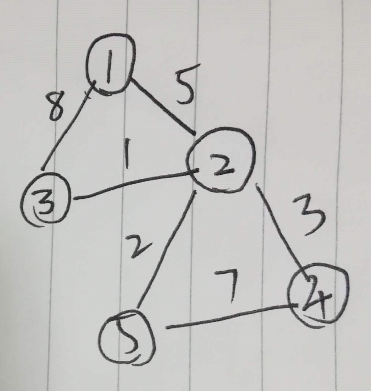
Sample Graph Data (Undirected)

The graph looks roughly like this:

How Dijkstra’s Algorithm Works

Dijkstra’s algorithm is essentially a greedy method:

Initialization We maintain two sets of vertices:
- Determined: vertices whose shortest distance from the source is finalized.
- Undetermined: the rest.
Pick the next vertex Among all undetermined vertices, pick the one u with the smallest tentative distance from the source, and mark it as determined.
Relax its outgoing edges For each neighbor v of u, update
```
dist[v] = min(dist[v], dist[u] + weight(u, v))
```

Step-by-Step Simulation

Let’s take 1 as the source and find the shortest distances to all vertices.

Setup
- dist[i] = tentative distance from i to source (initially ∞ for all except the source, which is 0).
- map[u][v] = weight of edge (u → v), or ∞ if no direct edge exists.
Initial state:
```
dist = [0, ∞, ∞, ∞, ∞]
determined = {1}
```
First iteration (start = 1)
- Relax edges out of 1:
  - map[1][2] = 5 → dist[2] = 5
  - map[1][3] = 8 → dist[3] = 8
- No edges to 4 or 5 from 1.
```
dist = [0, 5, 8, ∞, ∞]
next pick = vertex 2 (dist = 5)
```
Second iteration (start = 2)
- Relax edges out of 2:
  - map[2][3] = 1 → dist[3] = min(8, 5+1) = 6
  - map[2][4] = 3 → dist[4] = 8
  - map[2][5] = 2 → dist[5] = 7
```
dist = [0, 5, 6, 8, 7]
next pick = vertex 3 (dist = 6)
```
Continue until all vertices are determined After processing 3 and 4 similarly, no further updates occur, and we end up with:
```
dist = [0, 5, 6, 8, 7]
```
These are the final shortest distances from vertex 1.

C++ Implementation (Adjacency Matrix)

#include <iostream>
#include <algorithm>
#include <cstring>
using namespace std;

const int MAXN = 110;
const int INF = 0x3f3f3f3f;

int n, m;
int graph[MAXN][MAXN];
int dist[MAXN];
bool used[MAXN];

void dijkstra(int src) {
    // Initialize distances
    fill(dist, dist + n + 1, INF);
    memset(used, 0, sizeof(used));
    dist[src] = 0;

    for (int i = 1; i <= n; i++) {
        // Find the unused vertex with the smallest distance
        int u = -1;
        for (int v = 1; v <= n; v++) {
            if (!used[v] && (u == -1 || dist[v] < dist[u])) {
                u = v;
            }
        }
        used[u] = true;

        // Relax edges out of u
        for (int v = 1; v <= n; v++) {
            if (graph[u][v] < INF)
                dist[v] = min(dist[v], dist[u] + graph[u][v]);
        }
    }
}

int main() {
    cin >> n >> m;
    // Initialize graph with INF
    for (int i = 1; i <= n; i++)
        for (int j = 1; j <= n; j++)
            graph[i][j] = (i == j ? 0 : INF);

    // Read edges
    for (int i = 0; i < m; i++) {
        int u, v, w;
        cin >> u >> v >> w;
        graph[u][v] = w;
        graph[v][u] = w; // because undirected
    }

    dijkstra(1);

    // Output distances
    for (int i = 1; i <= n; i++)
        cout << dist[i] << " ";
    return 0;
}

Note: This version fails if there are negative edge weights. To handle negative weights, you’d need Bellman–Ford (or SPFA).

C++ Implementation (Adjacency List)

When using an adjacency list, the worst-case time complexity becomes O(n·m), which can be larger than O(n²) if the graph is sparse, but the space complexity drops from O(n²) to O(m).

#include <iostream>
#include <vector>
#include <queue>
#include <cstring>
using namespace std;

const long long INF = LLONG_MAX;
struct Edge { int to; long long w; };

int n, m, s;
vector<vector<Edge>> adj;
vector<long long> dist;
vector<bool> vis;

void dijkstra() {
    dist.assign(n+1, INF);
    vis.assign(n+1, false);
    dist[s] = 0;

    // min-heap of (distance, vertex)
    priority_queue<pair<long long,int>, vector<pair<long long,int>>, greater<>> pq;
    pq.push({0, s});

    while (!pq.empty()) {
        auto [d, u] = pq.top(); pq.pop();
        if (vis[u]) continue;
        vis[u] = true;

        for (auto &e : adj[u]) {
            int v = e.to;
            long long w = e.w;
            if (dist[v] > d + w) {
                dist[v] = d + w;
                pq.push({dist[v], v});
            }
        }
    }
}

int main() {
    cin >> n >> m >> s;
    adj.assign(n+1, {});
    for (int i = 0; i < m; i++) {
        int u, v; long long w;
        cin >> u >> v >> w;
        adj[u].push_back({v, w});
        adj[v].push_back({u, w}); // if undirected
    }

    dijkstra();

    for (int i = 1; i <= n; i++)
        cout << dist[i] << " ";
    return 0;
}

With a heap (priority queue) optimization, Dijkstra’s time complexity drops to O((n + m) log n), which for dense graphs (m ≈ n²) is better than SPFA.

A Personal Reflection

It’s been over a year—back when I first learned Dijkstra and adjacency lists, they seemed daunting. I even changed my handle to “Dijkstra” because I liked how it sounded! Over time I nearly forgot pure Dijkstra in favor of SPFA for negative edges.

Nowadays, with the heap-optimized version, Dijkstra runs in O(n log n). For dense graphs (e.g., a complete graph where m ≈ n²), n log n is still less than m, so the heap-optimized Dijkstra is the clear choice.